Troubleshooting Vibrating Wire Piezometers
通过 Nathanael Wright | 更新: 03/28/2023 | 评论: 0
博客主题


Product Category


搜索博客
订阅博客
出现新文章时获得邮件。选择您感兴趣的主题。
推荐文章
您是否想了解一个主题更多?请让我们知道。
Campbell Scientific vibrating wire measurement hardware, with our patented VSPECT™ technology, offers a distinct advantage over all other vibrating wire measurement systems. Unlike non-Campbell Scientific vibrating wire interfaces that use pulse counting to derive vibrating wire frequency, Campbell Scientific's VSPECT vibrating wire measurement products use spectral analysis to identify the sensor's resonant frequency, while rejecting interference and competing frequencies, to provide a superior measurement.
Even with superior technology, it can sometimes be difficult to answer questions such as these: Is my sensor unresponsive? Are the wires cut or broken? Am I getting a lot of interference?
To help us answer these questions, here are six parameters we’re going to use to check the readings:
- Sensor frequency
- Amplitude
- Signal-to-noise ratio
- Noise frequency
- Decay ratio
- Thermistor
All our VSPECT vibrating wire measurement products can read these values, including the CR6, CRVW3, Granite™ VWire 305, AVW200 Series, and the VWAnalyzer. For this discussion, I’ll be using the CR6 datalogger with the downloadable Device Configuration Utility application.
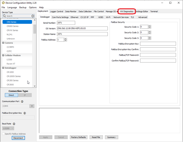
First, connect to your data logger using the Device Configuration Utility. After connecting, select the VW Diagnostics tab on the top row.
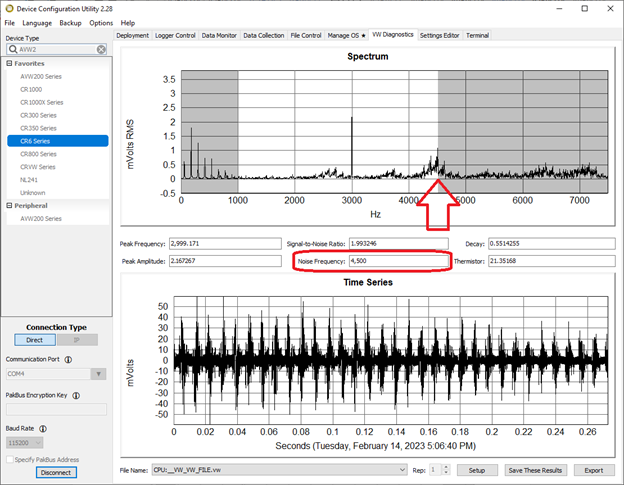
The image below shows the VW Diagnostics tab. In the middle, you can see the six fields that will contain the diagnostic values we’re going to use: Peak Frequency (for sensor frequency), Peak Amplitude (for amplitude), Signal-to-Noise Ratio, Noise Frequency, Decay, and Thermistor. When running the diagnostic test, the spaces both above and below these fields will populate with graphs that will help us contextualize the information visually.
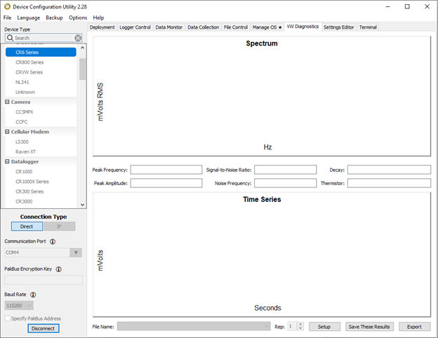
The information in the two graphs and the six fields will be populated automatically when the CR6 makes a measurement. Depending upon the measurement interval programmed in the data logger, there may be a delay before the data logger makes a measurement. If this happens, configure the data logger to store the information to a file that can be downloaded later. This file can also be useful if you want to show it to a technician for help with analysis.
Let’s go through the process now.
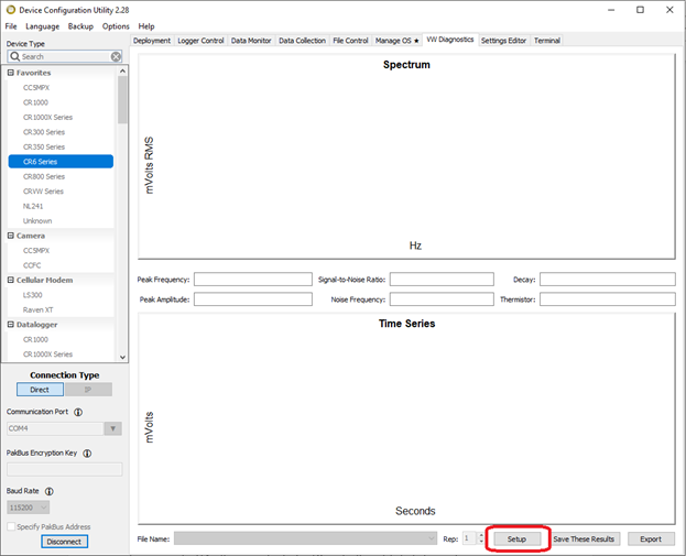
To begin, click Setup in the bottom right corner of the window. This displays the VW Diagnostic Setup window.
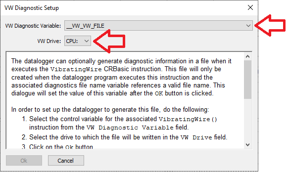
To configure the CR6 to generate the diagnostic file, click the VW Diagnostic Variable drop-down box and select the appropriate file name. In the VW Drive drop-down box, select the data logger storage drive to store the file on.
Note: Although these two fields are pre-populated, you must make selections in each of them, including entering a valid file name and location, before the Ok button will become available.
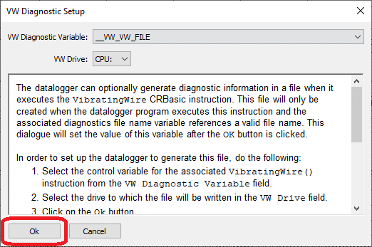
Click Ok. The data logger will measure the sensor, display the data on the screen, and store the data in the data logger’s file system. After the measurement is made, the file will be written to the selected drive and the file name will show up in File Control.
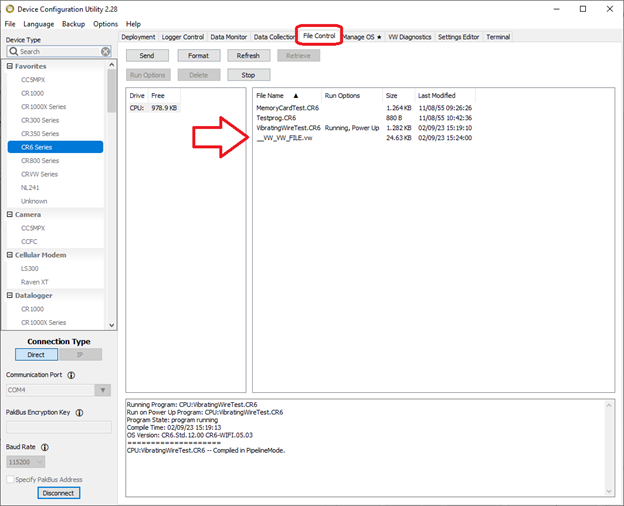
This file can be downloaded via File Control or exported from the VW Diagnostics tab by clicking either Save These Results or Export.
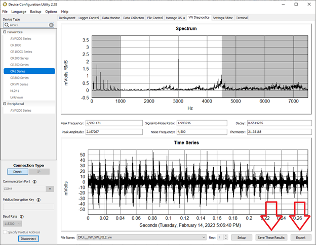
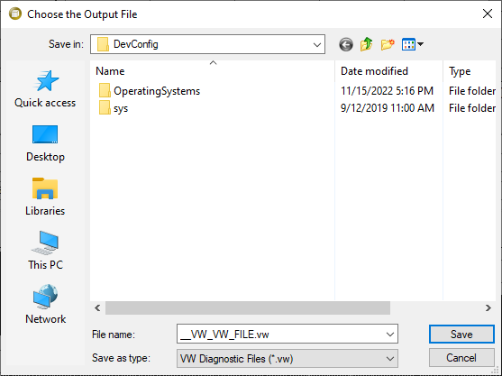
If you chose Save These Results, be sure to save the file in a place you can find again. Notice the .vw extension at the end of the file. This file contains the same spectrum and time series data you see in your live window and can be opened on any computer through the VW Offline Analysis mode of the Device Configuration Utility.
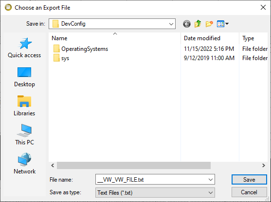
Alternatively, clicking Export prompts you to save a different type of file. Be sure to save it in a place you can find. Notice the .txt extension at the end of the file. This file can be opened in a text editor later to see a series of readings from the CR6.
To maximize what can be learned from diagnostics, you might consider saving both files every time. However, for purposes of this blog article, save only the .vw extension file (Save These Results) to allow us to see the data charted in the offline mode.
There’s no reason that you can’t do your analysis directly from the VW Diagnostics tab that you saved your .vw file from. But, offline mode is useful for when you go out in the field to check a large number of stations. You can save the files with unique station file names and do your analysis on all the stations at a later time.
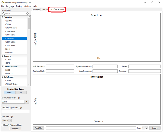
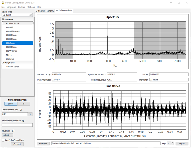
Now, let’s navigate to the VW Offline Analysis tab in the Device Configuration Utility.
Click Read File from the bottom left of the window.
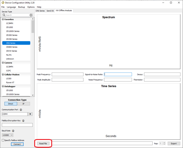
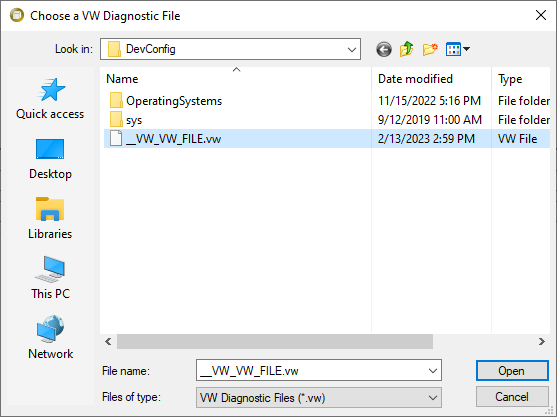
From the Choose a VW Diagnostic File window, select the .vw file that you saved previously and click Open.
Let’s look at a generic good reading on the graphs and compare it to what we see on the VW Offline Analysis tab.
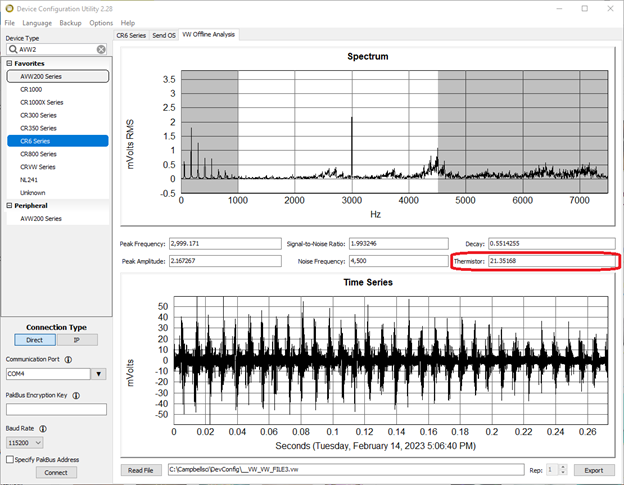
In my example here, I deliberately introduced 60 Hz AC line noise into my measurement by using a drill near the sensor when it was taking a reading. Environmental electrical interference, in typical installations, could be induced by AC power generation (e.g., a hydroelectric dam), by overhead high-intensity power lines, when sensor cables have to be shared in the same conduit with AC power conductors, for structural health monitoring (e.g., electric railway monitoring), and in construction applications where high-frequency welders are being used.
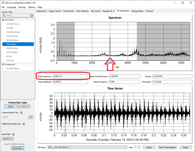
In analyzing the data, we can see the Peak Frequency (also known as the resonant frequency) field of the sensor. This is our measurement; its frequency is approximately 3000 Hz.
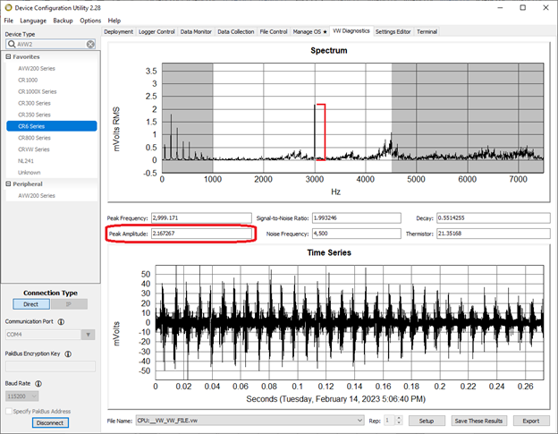
We also see the peak amplitude. The peak amplitude on the chart is the signal strength of our measurement.
Below we can see the noise frequency of the reading. Its peak has a frequency of 4500 Hz.
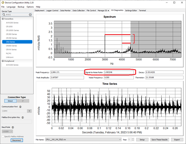
Next, consider the signal-to-noise ratio. It is the size of the space between the highest peak of the interference and the highest peak of the peak frequency (or resonant frequency). We can also refer to this as the measurement quality.
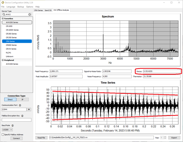
The decay ratio is the signal attenuation of the measurement. The number is easy to read from the Decay field. However, seeing it in the chart is difficult due to the unusual amount of interference added in the test measurement by my use of the drill. Generally, you can see below that the height of the wave on the left is a little taller than the one on the right. (For a much cleaner view, skip down to the isolated normal Time Series chart example a little further below.)
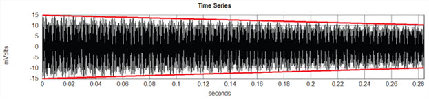
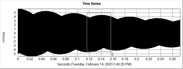
Here is an isolated normal Time Series chart example for decay with minimal interference:
The last parameter, the thermistor reading, is not indicated in the Spectrum chart on top nor in the Time Series chart below. Some vibrating wire sensors do not have a thermistor. If the sensor has a thermistor, the value will be displayed in either ohms or temperature in degrees Celsius. In our example, the displayed value is temperature.
Let’s consider one more detail before we talk about how to tell if the sensor is failing. In all the example charts, you may have noticed the two gray areas in the Spectrum chart. The white area in between the two gray areas is the sensor’s frequency range. The gray areas are the ranges that are going to be ignored in the actual measurement recording. This range allows us to ignore interference, reflections, or any frequency that the sensor is not going to respond to.
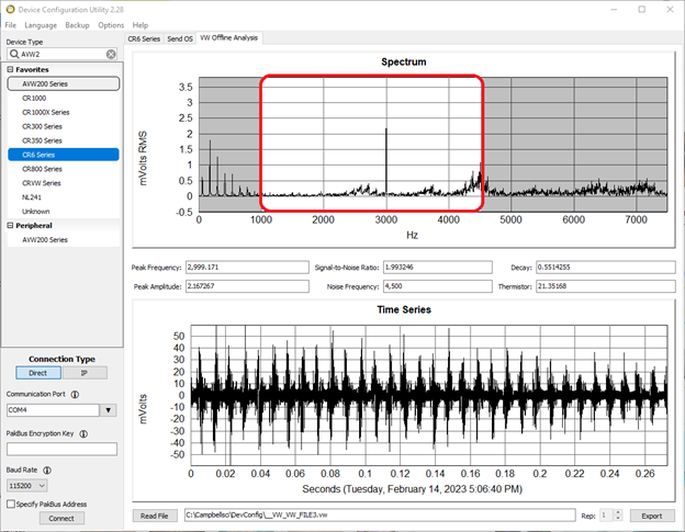
This range can be adjusted in your CRBasic code using the VibratingWire() instruction. Be sure to consult the manufacturer’s specifications for your sensor before making any adjustment to these parameters. Opening up the boundaries of the sweep frequency range can make your measurement susceptible to additional interference, and tightening the range can result in missed measurements. Here’s an example of the instruction:

Rules for Reading My Diagnostic Files
Now, I can hear you saying, “I’ve created a .vm diagnostic file. But how do I know if my vibrating wire sensor is bad?” To answer this question, I will first give you a few rules for knowing that something might be wrong with your measurement. Then, I will show you a few examples of measurements ranging from nearly flawless to a sensor with broken wires.
Rule #1
Check the frequency range of your sensor in the manufacturer’s specifications. Verify that the peak frequency you are receiving in your diagnostics falls within the manufacturer’s specifications.
Rule #2
If you are getting a NAN for peak frequency, you aren’t getting a measurement. This could be due to a broken sensor wire.
Rule #3
Check to see if the (peak) amplitude is greater than 1 mV RMS. If so, your measurement has good amplitude. If it's less than .02, the data logger will record NAN. Campbell Scientific data loggers can technically measure as low as .01 RMS, but due to the extremely weak signal being a problem, we set a threshold of .02 for the diagnostic parameter.
Rule #4
If your signal-to-noise ratio is really low (.1 or less), it can be difficult for the data logger to distinguish between a real measurement and noise.
Rule #5
If your noise frequency is really close to your measurement frequency, the data logger may see the noise as a measurement.
Rule #6
A good measurement has a decay that is somewhere near the middle of .50. If your decay is really high (e.g., .90) or really low (e.g., .10), then your sensor is likely starting to fail.
Rule #7
If your sensor does not have a thermistor or your sensor’s thermistor is deliberately not wired up, this value is OK being at NAN. If you are getting a really low value or a NAN and your sensor has a thermistor, the wires going to your sensor for the thermistor might be broken or the thermistor might be starting to fail.
Examples of Readings
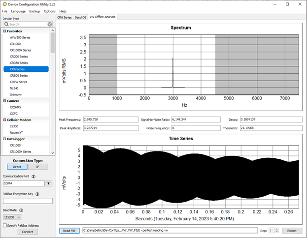
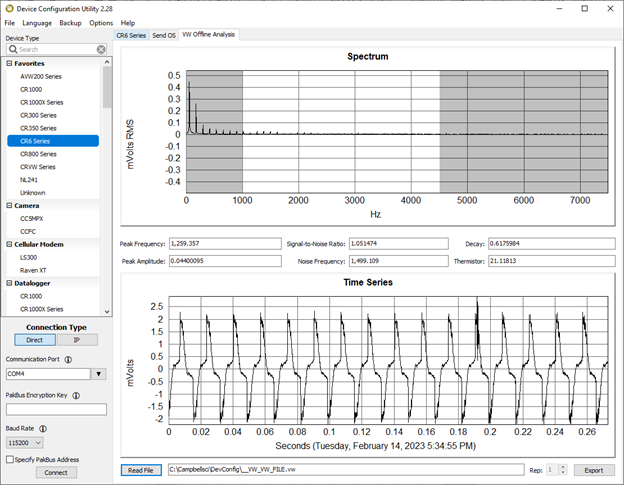
An excellent measurement
I’ve checked the Peak Frequency reading from my sensor and verified that the reading falls within the manufacturer’s specifications. That reading is not NAN. My Peak Amplitude is 3.22, which is well above the 1 mV threshold for high confidence in the strength of my reading. My Signal-to-Noise Ratio is high, indicating the dramatic difference between my peak frequency and noise frequency. This number is high because there is almost no noise, as indicated by the 0 value in the Noise Frequency field. My Decay reading at .589 is very near the middle range. Last of all, because my sensor has a thermistor, I can see a good value of approximately 21 °C for its value.
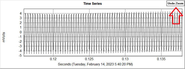
You might observe that the Time Series graph on the bottom is all black. I could maximize the Device Configuration Utility window to display the data better, or I can zoom in and look at things up close.
To zoom in, click and drag with your mouse. When you release your mouse button, the screen will zoom in on the Time Series chart. This zoom method also works on the Spectrum chart. To undo the zoom and return to your previous view, click Undo Zoom.
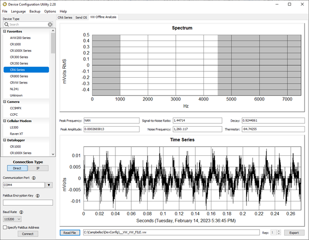
A sensor simulating broken or disconnected wires on the vibrating wire part of the sensor
You can see that the Peak Frequency appears to have a value that would fit into the range of the sensor. However, the Peak Amplitude is extremely low. If this reading was valid, it would be hard to differentiate it from noise based upon its extremely low amplitude. The Signal-to-Noise Ratio is also extremely low at roughly 1.05, indicating that it’s going to be difficult to differentiate any real reading from noise. Though the Noise Frequency value is approximately 150 Hz from the Peak Frequency, looking at the graph at the top, I can’t visually differentiate any of the little peaks from one another. This indicates that my Peak Frequency and my Noise Frequency are likely just noise. My Time Series chart on the bottom is made up of a bunch of little oddly shaped spikes, also indicating that it’s likely just noise. The one silver lining here is that my Thermistor reading is likely good.
A sensor simulating a completely severed wire
My first sign that something is wrong with this is that the Peak Frequency is NAN. My Peak Amplitude is so low as to make the value meaningless. My Signal-to-Noise Ratio is low. My Noise Frequency is of no consequence because everything else is bad. The Decay is high but irrelevant since the Peak Amplitude is so low that any Time Series data isn’t going to reflect my measurement. The Thermistor is returning a value of roughly -94 °C, indicating a problem with that reading as well. I know that I should be expecting something close to 20 °C for the environment I’m currently in. I would draw the same conclusion if the Thermistor reading was NAN.
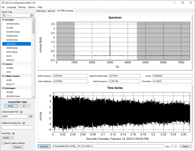
A very good sensor reading with slight interference
Looking at the Spectrum graph, we can see the little spikes on the bottom of our reading. But the Peak Frequency is very clearly defined. The bottom Time Series looks normal except for small spikes at the top and bottom, which indicate the little bit of noise we are seeing. The Peak Frequency value looks good, and the Peak Amplitude is greater than 1 mV. The Signal-to-Noise Ratio isn’t perfect, but there is enough to indicate that we should get a clear reading. The Noise Frequency peak is far enough separated from the Peak Frequency to easily differentiate it. The Decay is near the middle, and the Thermistor reading looks valid. If my sensor did not have a thermistor, a value of NAN would be acceptable here.
Final Thoughts
I hope this explanation, the accompanying rules, and the examples have been helpful. Campbell Scientific’s VSPECT technology helps eliminate noise and competing frequencies from your vibrating wire measurements, and is vastly superior to non-Campbell Scientfic vibrating wire interfaces. With our diagnostic tools, it can be much easier to determine the cause of a measurement problem. There really is nothing quite like VSPECT in the industry.
If you have any questions or comments, please post them below.


关于作者
 Nathanael Wright is a Technical Support Specialist at Campbell Scientific, Inc. He provides technical support for data loggers, instruments, and communications equipment. Nathanael has a bachelor's degrees in Computer Information Science and Business Administration, and an MBA. In addition, Nathanael has more than 15 years of experience working in IP communications. Away from work, he enjoys breakdancing, hiking, writing, publishing books, and fiddling with computer equipment.
建议
Please log in or register to comment.